Part 1: Method overview
In the field of metagenomics data analysis, there is an endless universe of pipelines or methodologies you can follow to explore and characterize your samples. We recommend this comprehensive review for you to explore the different existing approaches. For this course, we propose to wrap with Nextflow the protocol published by Jennifer Lu et al. (2022).
The example dataset we will use to demonstrate the analysis consists of only paired-end reads recovered from an oligotrophic, phosphorus-deficient pond in Cuatro Ciénegas, Mexico (Okie et al.,2020) in FASTQ format. The BioProject accession number is PRJEB22811.
1. Workflow design
Our goal is to develop a workflow that takes FASTQ files from one or multiple samples as input and applies the following processing steps: host removal, taxonomic classification, Bayesian re-estimation of species abundance, and generation of plots and metrics.
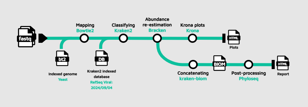
To perform these steps, we will use the following tools:
- Host removal with Bowtie2 by aligning the reads against an indexed reference genome. Here, we are using the indexed genome of yeast given the computational limitations we have on GitHub Codespaces and only for educational purposes. Nonetheless, you can use any organism you are interested in by building your own index or downloading a precomputed one.
- Taxonomic classification with Kraken2. This tool relies on an indexed database that can be downloaded. Alternatively, you can build your customized version following these instructions. Here, we will use the Viral database, therefore this methodology is labeled as "viral metagenomics". However, you can annotate bacteria, archaea and more simply by switching to another database.
- Bayesian re-estimation of species abundance with Bracken. This software is designed to compute species abundance using Kraken classification results as described in the reference paper. It also uses some files contained in the database folders such as the kmer distribution files. This is a fairly complex analysis, but you don't need to know the details in order to follow this tutorial; you can learn about how the method works afterwards.
- Plot generation with Krona from the Bracken output. This will allow us to visualize interactively the relative abundance of each annotated species.
- (Multi-sample) Concatenation with kraken-biom. If multiple samples are provided, the Bracken reports will be concatenated and converted into a Biological Observation Matrix (BIOM) file.
- (Multi-sample) Generation of final report with Phyloseq
The BIOM file will be converted to a Phyloseq object, and this object will be further processed to generate absolute plots, estimate both α and β-diversity and perform a network analysis.
This information will be presented in a final
report.html. To learn more about the code used to generate the plots and metrics, check out this Phyloseq tutorial.
Tip
If you feel a bit overwhelmed by the theoretical background of the methodology, we strongly encourage you to check this Carpentries lesson first, where the concepts are explained step by step using interesting examples.
2. [TODO: add optional manual testing of the various tools via containers]
Takeaway
You understand the underlying method and the overall design of the workflow.
**[TODO: You have tested all the individual commands interactively in the relevant containers.] **
What's next?
Learn how to wrap those same commands into a multi-step workflow that uses containers to execute the work.